Math foundations
The Binomial Distribution: Counting Successes in n Trials
The idea
Flip a biased coin ten times, run ten identical ad impressions, ship ten deploys. Each trial is an independent yes/no event with the same success chance p. The binomial distribution tells you the probability of getting exactly k successes across all n trials — not just the average, but the full shape of what could happen.
The binomial answers: across n independent tries at rate p, how likely is each possible count of successes?
Example: successes in n independent trials
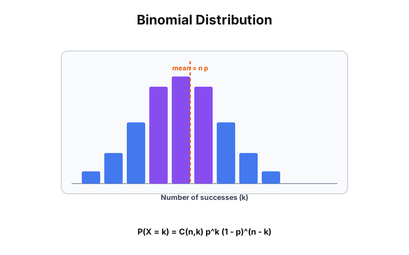
Set the number of trials and the success chance per trial. Each bar is the probability of seeing exactly that many successes. The orange line marks the expected count, n · p.
Mean (n·p)
5.00
Std dev
1.58
Peak at k
5
P = 24.6%
Across 10 independent trials at 50% each, expect about 5.0 successes, give or take 1.6. The single most likely count is 5. Spread is widest at p = 50% and shrinks as p heads toward 0 or 1.
The math
Probability mass function
C(n, k) counts the number of arrangements of k successes among n slots (see combinations). p^k is the chance of those successes; (1 - p)^(n-k) covers the failures.
Mean and variance
The expected count scales linearly with n. Spread is largest at p = 0.5 and vanishes as p approaches 0 or 1, because near-certain trials have little to vary.
A simple application
If a checkout flow converts 8% of the time and you get 200 visitors, the binomial says how many purchases to expect and how noisy that count is — the foundation for reading a thin sample size or a win rate. Sum many binomial trials and the count starts to look like a normal distribution; keep p tiny while n grows and it becomes Poisson.