Math foundations
The Normal Distribution: Bell Curves, Mean, and Standard Deviations
The idea
Many operational metrics cluster around a center with symmetric tails: delivery times, order values, measurement error. The normal distribution models that shape with two parameters: mean mu and standard deviation sigma.
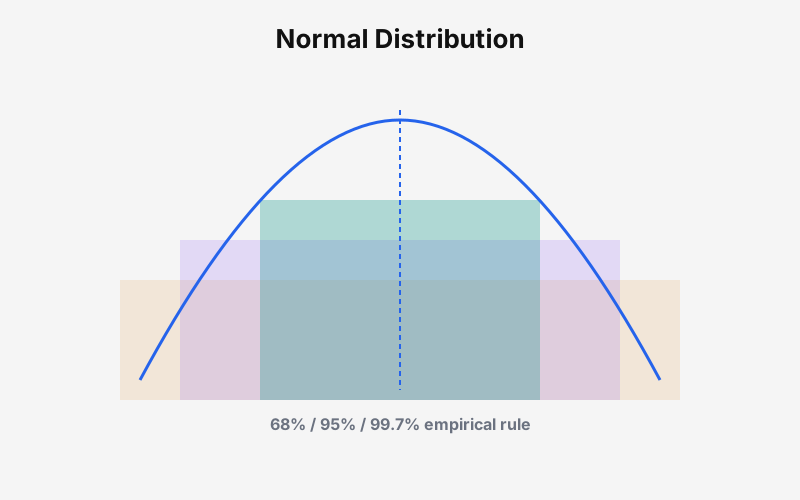
The empirical rule gives fast mental math: about 68% of mass within one sigma, 95% within two, 99.7% within three. Z-scores count how many standard deviations a value sits from the mean, linking this curve to feature scaling and outlier checks.
Normal is a working model, not a law of nature. Check fit before you trust tail probabilities.
Example: bell curve, mean, and sigma bands
The normal density clusters around mu. Sigma sets spread. Shaded bands show the 68-95-99.7 empirical rule in action.
Most orders cluster near the mean. Sigma sets how wide the bell spreads.
+/-1 sigma
68%
+/-2 sigma
95%
+/-3 sigma
99.7%
Mean 45.0 min, sigma 8.0 min. About 68% fall within +/-1 sigma, 95% within +/-2, and 99.7% within +/-3 when the normal model fits.
The math
Probability density function
Bell-shaped density centered at mu. Sigma stretches or tightens the curve. Total area under the curve equals 1.
Empirical rule
Quick coverage bands for roughly normal data. Useful for SLA bands and anomaly thresholds when you have not plotted the full distribution yet.
Z-score link
Standardizes any normal variable to mean 0, sigma 1. Connects this post to feature scaling and to asking how extreme one observation is.
A simple application
When you set an alert at mu + 3 sigma, you are assuming normality and targeting roughly 0.15% tail mass on the high side. Plot the histogram first. Heavy tails or skew mean the normal approximation will miss real outliers or over-flag routine noise.
Use the normal model for quick capacity planning and error budgets. Pair with variance-spread and percentile posts when the data is not symmetric.