Math foundations
Logarithms and Odds: Why Log-Odds Show Up in Logistic Models
The idea
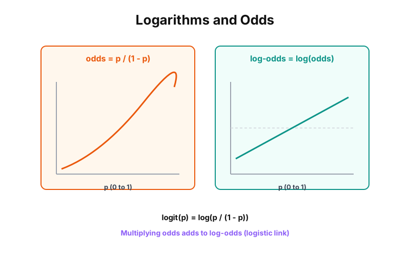
Probability p lives between 0 and 1, but models want an open real line. Odds p / (1 - p) stretch as p nears 1. The logarithm of odds (log-odds, or logit) turns multiplicative shifts into additive ones. That is why a linear score z = w · x maps cleanly to a probability through the sigmoid.
Log-odds answer: How do we keep probabilities bounded while staying linear in features?
Example: probability, odds, and log-odds on one slider
Probability lives on (0, 1). Odds stretch to infinity as p approaches 1. Log-odds turn multiplication into addition, which is why logistic models stay linear in features.
e^w = 1.65 (odds multiplier)
odds = p / (1 - p)
0.67
log-odds = log(odds)
-0.41
+ w = 0.09 → p = 52%
p
40%
odds
0.67
log-odds
-0.41
At p = 40%, odds = 0.67 and log-odds = -0.41. Adding feature weight w = 0.50 multiplies odds by e^w = 1.65 and adds w to log-odds → 0.09 (p = 52%). Logistic regression is linear in log-odds.
The math
Logarithm and change of base
Natural log (ln) is the default in ML. Change-of-base rewrites the same number in any log scale. Only the units change, not the relationships.
Odds
p = 0.5 gives odds 1 (even). p = 0.8 gives odds 4 (four wins per loss). Odds blow up as p approaches 1.
Log-odds
logit maps (0, 1) to all real numbers. Adding w to log-odds multiplies odds by e^w. Features combine by addition on the log scale.
Sigmoid inverse
Logistic regression sets z = w₀ + w₁x₁ + … and reads p from the sigmoid. z is the log-odds; the sigmoid is its inverse. See the logistic regression post for the full classification picture.
A simple application
A churn score starts at 20% (odds 0.25, log-odds -1.39). A usage feature with weight 0.7 multiplies odds by e^0.7 ≈ 2.0 and adds 0.7 to log-odds. Reading coefficients as odds multipliers is often clearer than reading raw probability bumps.