Math foundations
The Central Limit Theorem: Why Averages Go Normal
The idea
Individual data is messy: revenue is skewed by whales, latency has a long tail, sessions cluster. But when you take the average of a batch and repeat, those averages pile up into a smooth bell curve — even though the raw data was nothing of the sort. That is the central limit theorem, and it is why so much of statistics can lean on the normal distribution.
The CLT answers: why does the distribution of a sample mean look normal, no matter the shape of the underlying population?
Example: a lopsided population, a bell-shaped average
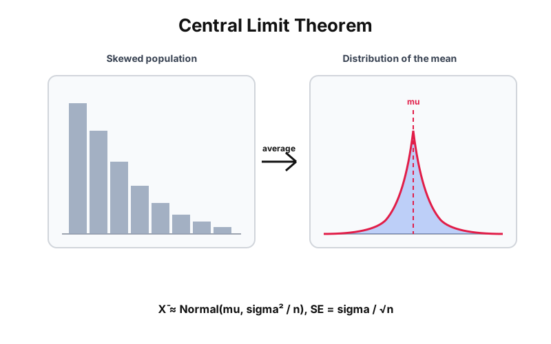
Pick any population shape on the left. The right panel is the distribution of the sample mean when you repeatedly average n draws. Raise n and watch it tighten into a bell.
Center of both
0.26
Population mean, unchanged by averaging.
Spread shrinks by
÷ √10 ≈ 3.16
Standard error = sigma / sqrt(n).
The population is skewed (long tail), yet averaging 10 draws pulls the distribution of the mean toward a symmetric bell. Its center stays at the population mean, and its spread shrinks with the square root of 10.
The math
Distribution of the mean
Draw n independent values with mean μ and variance σ². The sample mean X̄ is approximately normal, centered at the true μ, regardless of the population's shape.
Standard error
The spread of the sample mean shrinks with the square root of n. To halve your uncertainty you need four times the data — the reason precise estimates get expensive.
A simple application
The CLT is the engine under confidence intervals and A/B test readouts: it lets you put a normal-shaped range around a conversion rate or an average order value. It also explains why a bigger sample size tightens the read, and why the normal distribution shows up everywhere.